
Unbalanced Forces Lab (10/26/2021)
Ryan Rong, Priyanka Nanayakkara, Jenna Kim
Research Questions
1) How does the net force of the cart affect its acceleration
2) How does the total mass of a system affect its acceleration?
In the labs:
1)
The independent variable is the net force upon the cart, in Newtons.
The dependent variable is the acceleration of the cart, in m/s/s.
Control variables include the total mass of the cart and hanger system. Other controls include the hanger, the track and the cart.
We keep the total mass constant because the more mass an object has, the more its inertia and resistance to change in motion (acceleration) it has. To change the net force, move the weights from the cart to the hanger and keep the total mass constant instead of adding mass to the hanger.
2)
The independent variable is total mass of the system, in kg.
The dependent variable is the acceleration of the cart, in m/s/s.
Control variable is the net force acted upon the cart (or the mass of the hanger) since net force also affects acceleration asides from mass. Other controls include the hanger, the track and the cart.
Collection of data
We used a motion sensor to measure the velocity of the cart and used logger pro to calculate the acceleration of the cart in both experiments.
Lab setup
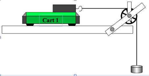
(Figure 1)
A string with one end attached to a cart passes through a pulley and is attached to a hanger on the other end. The cart slides on a leveled ramp and the motion sensor is fixed at the end of the ramp for both experiments.
Procedure
Lab 1:
- Position the cart at the end of the ramp and hold on to it.
- Start the motion sensor.
- Let go of the cart and let it slide across the ramp.
- Stop the cart with both hands before the hanger hits the ground.
- Record the total mass of the hanger (or net force)
- In logger pro, select the portion of the velocity time graph generated by the motion sensor from when the cart begins to accelerate to when the cart stops. Press "linear fit" and collect the linear coefficient (the acceleration of the cart).
- Repeat the previous steps for different masses on the hanger. Remember to keep the total mass constant.
Lab 2:
In addition, we used a scale to measure the cart which was 495 grams in both labs, and we did one trial for each net force in lab 1 and one trial for each mass of cart in lab 2.
- Position the cart at the end of the ramp and hold on to it.
- Start the motion sensor.
- Let go of the cart and let it slide across the ramp.
- Stop the cart with both hands before the hanger hits the ground.
- Record the mass of the cart.
- In logger pro, select the portion of the velocity time graph generated by the motion sensor from when the cart begins to accelerate to when the cart stops. Press "linear fit" and collect the linear coefficient (the acceleration of the cart).
- Repeat the previous steps for different masses on the cart. The total mass of the system changes but the mass on the hanger should be constant.
In addition, we used a scale to measure the cart which was 495 grams in both labs, and we did one trial for each net force in lab 1 and one trial for each mass of cart in lab 2.
Raw Data
Lab 1)
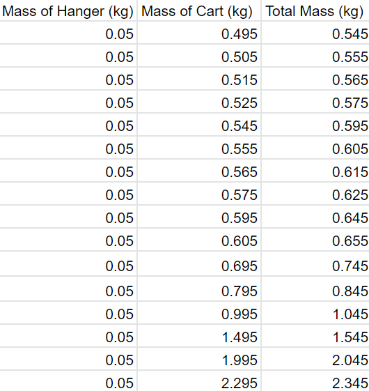
The mass of the cart is 0.495 kg. The total mass of the system is 0.675 kg.
The mass of the cart is 0.495 kg. The total mass of the system is 0.675 kg.
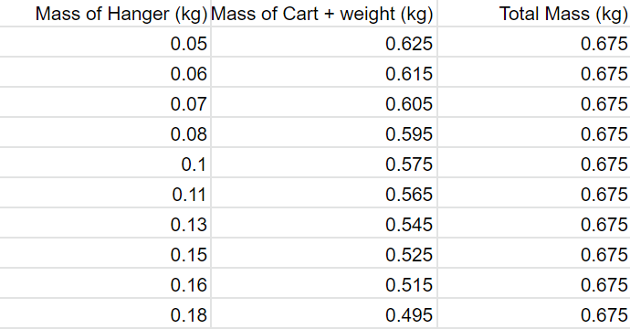
(Figure 2)
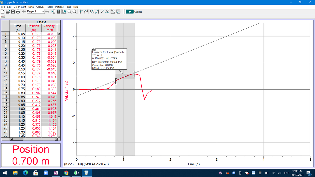
(Figure 3)
Figure 2 shows the how the weights were distributed between the cart and the hanger in each trial. Figure 3 is an example of the velocity time graph that the motion sensor generates (this example is when mass of hanger is 0.1 kg).
Lab 2)
The mass of the hanger is constant at 0.05 kg.
Lab 2)
The mass of the hanger is constant at 0.05 kg.
(Figure 4)
Processed Data
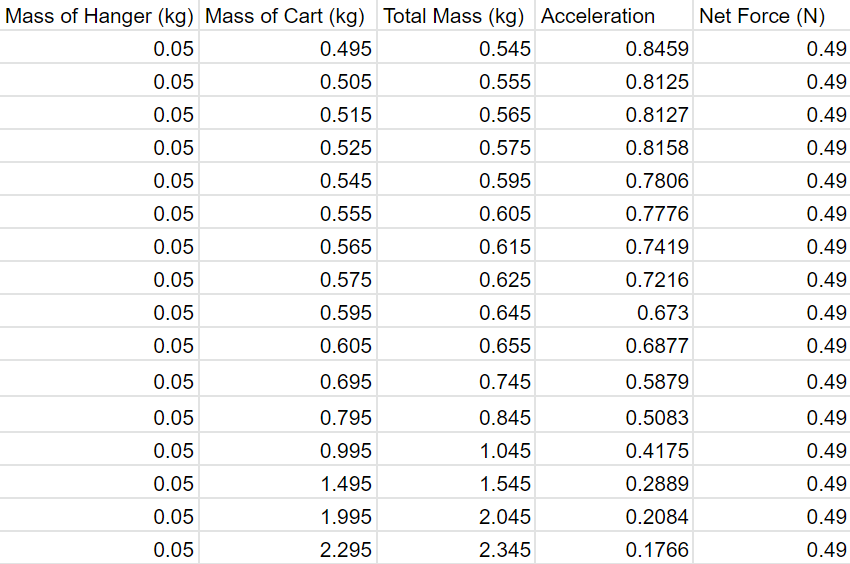
Lab 1)
(Figure 5)
In the processed data, the acceleration was calculated from the velocity graph in logger pro as described in "Procedures" above. The net force that acts upon the cart is a tension force from the string in the left direction. This tension force is generated by the the force of gravity on the hanger. Thus the net force is the force of gravity on the hanger, which is calculated by the equation Fg = mg where m is the mass of the hanger and g is the acceleration due to gravity (g=9.8)
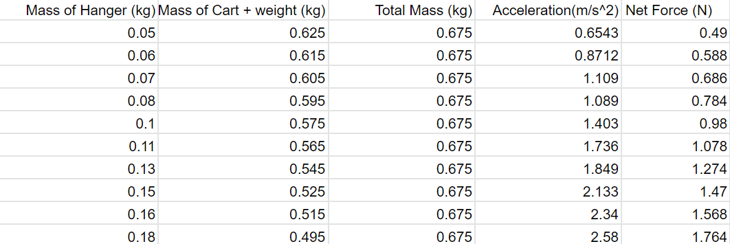
Lab 2)
(Figure 6)
In the processed data, the acceleration was calculated from the velocity graph in logger pro as described in "Procedures" above just like lab 1. The net force that acts upon the cart is still calculated by the equation Fg = mg as described above. In this case, the net force is constant at 0.49N since the mass of hanger is constant at 0.05 kg.
Graphs
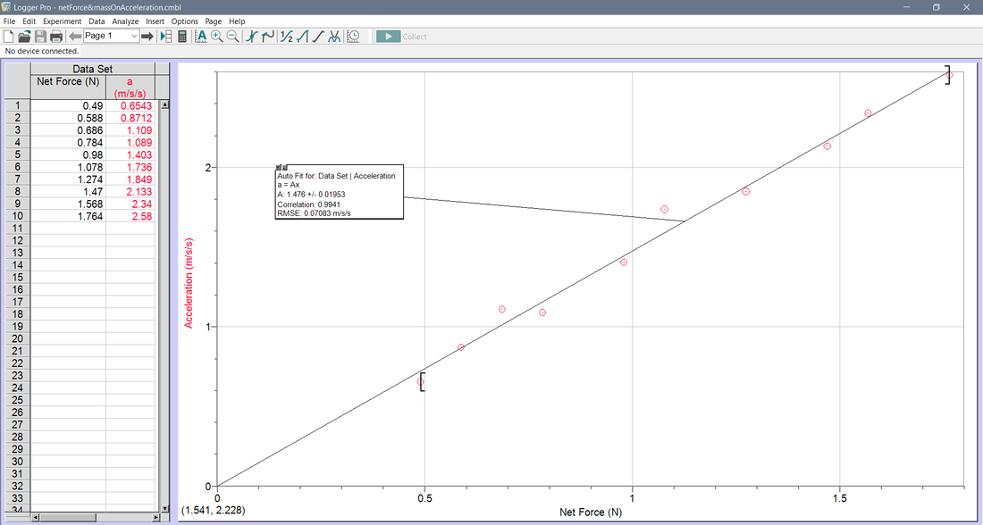
(Figure 7)
(Figure 8)
Figure 7 shows the results of lab 1. This graph shows how the net force acted upon the cart affects the acceleration of the cart. Logically, when there is a net force of zero acted upon the cart, its acceleration would be zero, which is why I chose a proportional fit for the data set where the y-intercept is zero. The equation of this model is Acceleration = 1.476 * ∑F. The slope of the graph is positive and constant at 1.476 m/s/s. This means that for every Newton of increase in net force, the acceleration increases by 1.476 m/s/s.
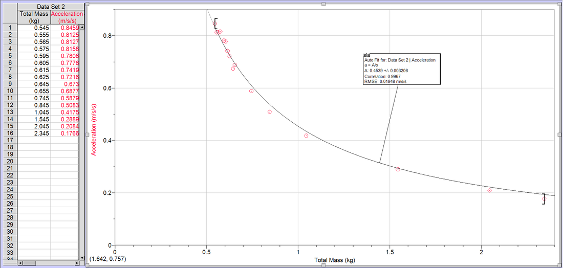
Figure 8 shows the results of lab 2. This graph shows how the total mass of the system affects its acceleration. Again, thinking logically, when the mass of the system is zero, there is nothing to accelerate. The acceleration would be undefined. Thus there is no y-intercept. The model for this lab is an inverse model with the equation Acceleration = 0.4539/mass. The inverse model does not have a constant slope but as the total mass of the system increases, the acceleration decreases by less and less.
Figure 8 shows the results of lab 2. This graph shows how the total mass of the system affects its acceleration. Again, thinking logically, when the mass of the system is zero, there is nothing to accelerate. The acceleration would be undefined. Thus there is no y-intercept. The model for this lab is an inverse model with the equation Acceleration = 0.4539/mass. The inverse model does not have a constant slope but as the total mass of the system increases, the acceleration decreases by less and less.
Purpose & Conclusion
Together, the two labs help us to prove Newton's Second Law of motion that Net Force = Mass * Acceleration. From our graphs, we can conclude that the acceleration of an object is dependent upon the Net Force acting on upon the object and the Mass of the object. In lab 1, the proportional model shows that Acceleration = A * ∑F, we can see that A = 1/mass as 1.476, the estimate made by the graph, is close to the actual value of 1/0.675. In lab 2, the inverse model shows that Acceleration = B/mass, we can see that B is the net force as 0.4539, the estimate made by the graph, is close to the actual value of 0.49N. Thus we can conclude that Acceleration = ∑F/m and changing the subject, ∑F = Acceleration * mass. As the force acting upon an object increases, the acceleration of the object increases. As the mass of an object increases, the acceleration of the object decreases, which makes sense as a heavier object is harder to accelerate than a lighter object.
Newton's Second Law is very powerful. It connects acceleration with mass and forces and can be used to describe a lot of motion in our everyday lives.
Newton's Second Law is very powerful. It connects acceleration with mass and forces and can be used to describe a lot of motion in our everyday lives.
Evaluation
Lab 1)
One source of uncertainty in this experiment was the range of the data. Due to the constraint that we could not have the cart accelerating too fast, we did not have large net forces acting on it. Another uncertainty was the exact time that the cart begins to accelerate/stops. The portion of data we selected on logger pro that calculated the acceleration of the cart might be a little bit off. Another uncertainty was air resistance as the force applied on the cart by air does play a role in every single trial. The friction of the tracks (which was minimal) also plays a role in the force applied on the cart, but both these forces are negligible for the purposes of the lab.
Lab 2)
Better than lab 1, the range of data we collected was relatively large. But same as lab 1, the portion of data we selected on logger pro that calculated the acceleration of the cart might be a little bit off. Another uncertainty that remains in both labs is that there were no multiple trials. We could have made small mistakes in individual trials, which led to inaccuracies.
Improvements
Lab 1)
With the sources of uncertainty being said in the previous section, one way to improve the investigation is to collect a larger range of data. It is always beneficial to have a bigger collection of data so we can fit the model much accurately. We can also conduct multiple trials for each net force to minimize the uncertainty from manual errors like the selection of when the cart begins to accelerate/stop.
Lab 2)
One way to improve our accuracy is, again, conduct multiple trials for each total mass to minimize the uncertainty from manual errors like the selection of when the cart begins to accelerate/stop.
